Optimising LP Performance Part 2: Dynamic Fees

In our previous article in this series, we discussed various metrics that LPs can employ to estimate the profitability of providing liquidity to AMM pools. This enables them to fine-tune their LPing strategies for a better net return in their portfolios. We also discussed how a metric like Impermanent loss is an inherent characteristic of CFMMs and cannot be avoided and thus we wish to focus our efforts on finding solutions to minimize the LVR of LP positions.

In the upcoming articles, we'll explore potential solutions aimed at enhancing LP profitability and mitigating the negative effects of LVR. These solutions for reducing LVR impact fall into several categories:

1. Dynamic Fees.
2. Protocol-level optimizations for AMMs, including on-chain Orderbook infrastructure.
3. Application-level improvements for AMMs and Hooks.
4. Batch Auctions, RFQs, and Intent-based solutions.

Teams are also working on countering the divergence loss experienced by LP positions through the solutions mentioned above and by hedging LP portfolio exposure. Many blockchain-based AMM implementations typically employ a constant fee approach for their liquidity pools. However, this approach fails to protect liquidity providers during turbulent market conditions, as it tends to:

• Price fees too low in volatile markets (as observed by liquidity shrinkage on order book exchanges during such periods).
• Price fees too high during stable periods, making decentralized exchanges less competitive against centralized counterparts in terms of fee-adjusted swap rates.

One of the most discussed solutions involves implementing dynamic fees for each liquidity pool. This approach either incentivizes flow to the pool during periods of low volatility or transaction volume or increases fees to compensate LPs during periods of high price volatility. In this article, we will explore some intriguing dynamic fee concepts we've encountered.

Multivariate Dynamic Fees

The building of this model of dynamic fees was suggested by the Ambient Finance team and uses a simple strategy utilizing historical data and predictive power of the previous time intervals to select the optimal fee in the next time interval. 

The construction of this dynamic fee policy starts with a lookback model executing a simple algorithm. 

1. For a given time interval of 10 minutes, determine which fee tier (out of the Uniswap 0.05%, 0.3%, and 1% pools) had the highest fee growth in each of the last 3 time intervals.
2. Use all available historical data to determine the highest-payoff selection of the next fee tier for the current time interval, conditional on the historical data in step 1.

Explaining the above algorithm

Suppose, we are only allowed to observe the best-performing fee tier for the latest time interval. The space of possibilities is quite limited (in fact, with 3 fee tiers there are only 9 possible models with a lookback window of 1 time interval).

On completing an examination of the “transition probabilities” of moving from fee tier X at time t-1 to optimal fee tier Y at time t the team realized regardless of the fee tier at time t-1, the most likely highest fee-generating tier at time t was the 0.05% pool rather than the 0.3% or the 1% pool. 

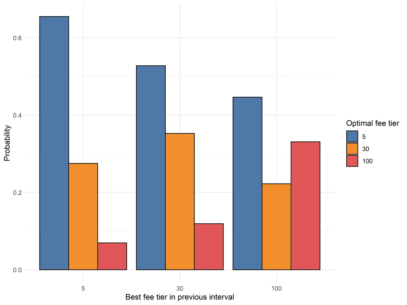
But this outperformance of 0.05% fee tier in most cases was due to the 0.05% pool facilitating the most volume each time period. We need to note and adjust our predictions with the information that it outperforms other fee tiers by only a very small margin as compared to when the 0.3% pool or, especially the 1% pool experiences strong fee accrual. 

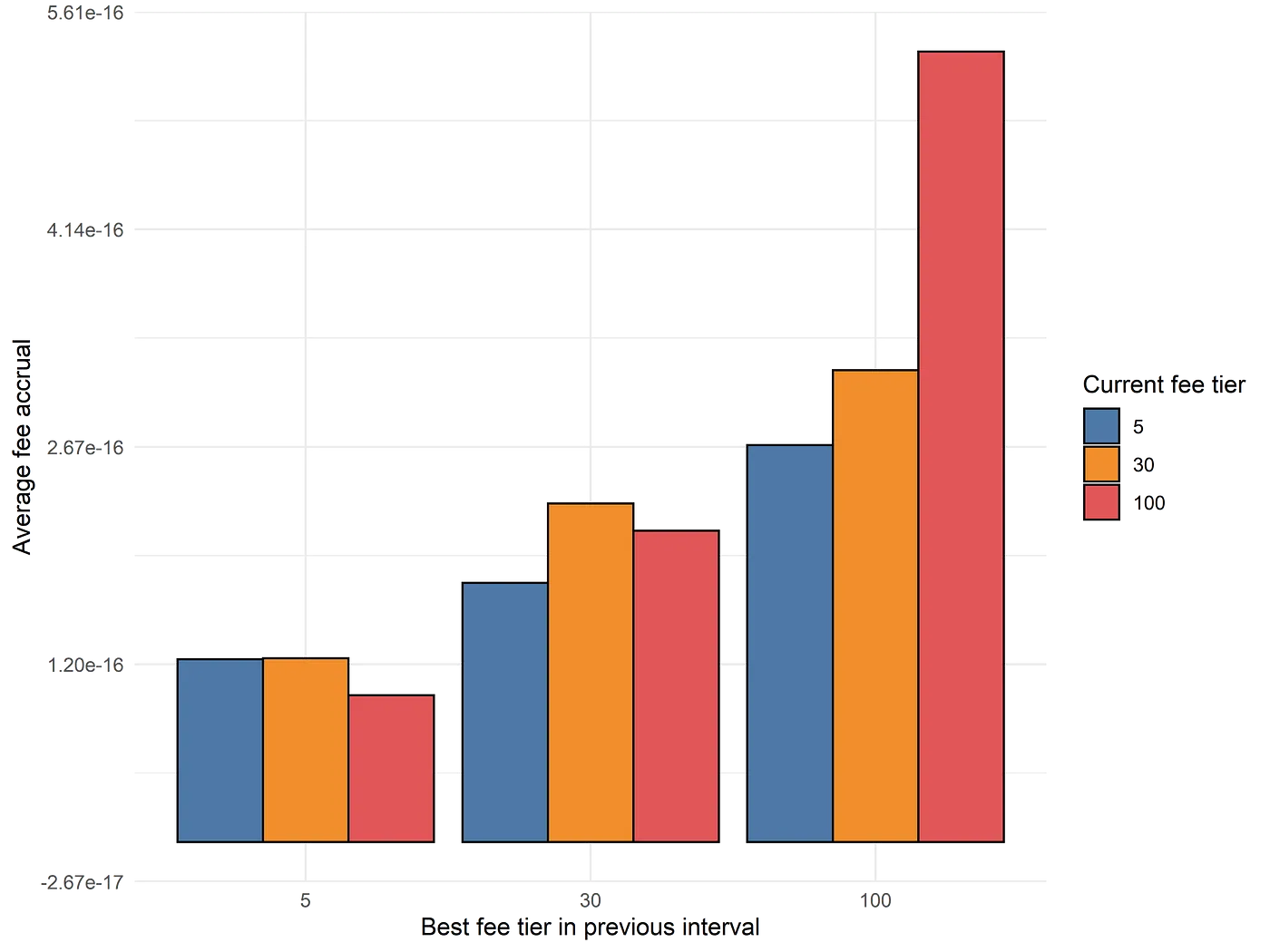
 Thus by adjusting the model to account for both factors: 

1. Probability of outperformance and 
2. Relative size of outperformance 

It turns out that simply “copying” the fee tier in interval T over to interval T+1 is quite close to optimal, within this limited model space. This matches a basic general intuition that higher fee tiers perform better in volatile environments, where the fee accrual of the 0.3% or 1% pools spikes due to an acute increase in the overall demand for liquidity.

Additionally, if a fee tier of 1% is optimal for interval T, the returns by selecting the 1% fee tier again for T+1 interval are quite high. Thereby suggesting the high value in accurately detecting the persistence of the highly volatile periods.

Extended Lookback 

After capturing the signal of one-period lookback, the next obvious question is to determine the signal value extractable from two-period, three-period and n-period lookback strategies. Just to briefly explain the difference between the one and two-period lookback we can think of it as follows - If the optimal fee tiers at t-2, and t-1 periods were 1%, and 0.3% respectively the one-period lookback would suggest 0.3% as the optimal fee. In contrast, the data from a 2-period lookback can end up predicting a 1% fee to outperform other fee tiers.

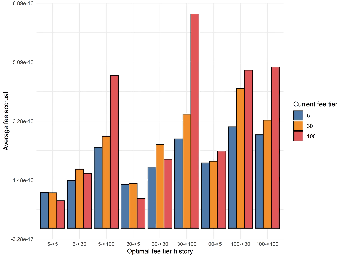
As mentioned earlier, the choice of optimal fee tier to be selected for the next time period is based on two criteria conditional on the observed fee accrual history

1. Probability that a given fee tier will be the best-performing fee tier
2. Returns achieved on correctly selecting that fee tier. 

These 2 factors are computed over all available historical data and then multiplied together to determine the expected payoff of selecting a given fee tier, conditional on the observed fee accrual history.  

  As we can see, it is natural to suspect that extending the lookback model even further back in history will only yield very marginal returns. The team then explored the idea of incorporating other variables into the analysis to generate superior performance. 

Extension of the model

The Ambient finance team added a variety of variables into their model, used different predictive modelling, changed the retraining frequency from daily to a monthly time-frame, and transformed the v4 lookback into 27 binary variables of difference in fee accrual of the 3 fee tiers, turning continuous variables into percentile bins, outlier removals, logarithmic transformations etc. We highly recommend reading the dynamic fee series from the team to better understand the nuances of creation and fine-tuning of the model.  

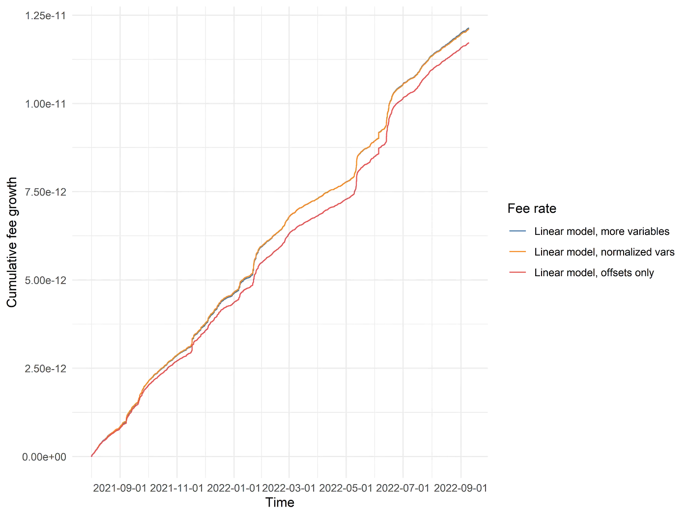
Surprisingly, there were no consistent transformations which substantially improved predictive power over simply plugging in the predictor variables into a simple linear model. After running a linear regression model across a variety of parameters, transformations and pairwise relationships they picked the following combination of 5 predictors which work well in practice

1. Swap volume in USD, in the previous time interval
2. Maximum price tick minus minimum price tick, in the previous time interval
3. Number of swaps, in the previous time interval
4. Standard deviation of the price tick across different swaps, weighted by swap value in USD, in the previous time interval
5. Interaction of the difference in fee accrual with a categorical variable encoding the highest-performing fee tier, in each of the three most recent time intervals

Note that we are not interested in swap volume or the number of swaps in T-1 time interval directly so much as we are interested in volume and swap count relative to recent history. That is we need to ascertain if swap volume or activity in a given time interval is abnormally high or low relative to swap volume or activity in the last week or the last month. To do so the Ambient Finance team used to divide the raw values of interval T-1 by the average swap volume or swap count across time intervals in the last month (normalizing the variables to a certain extent).

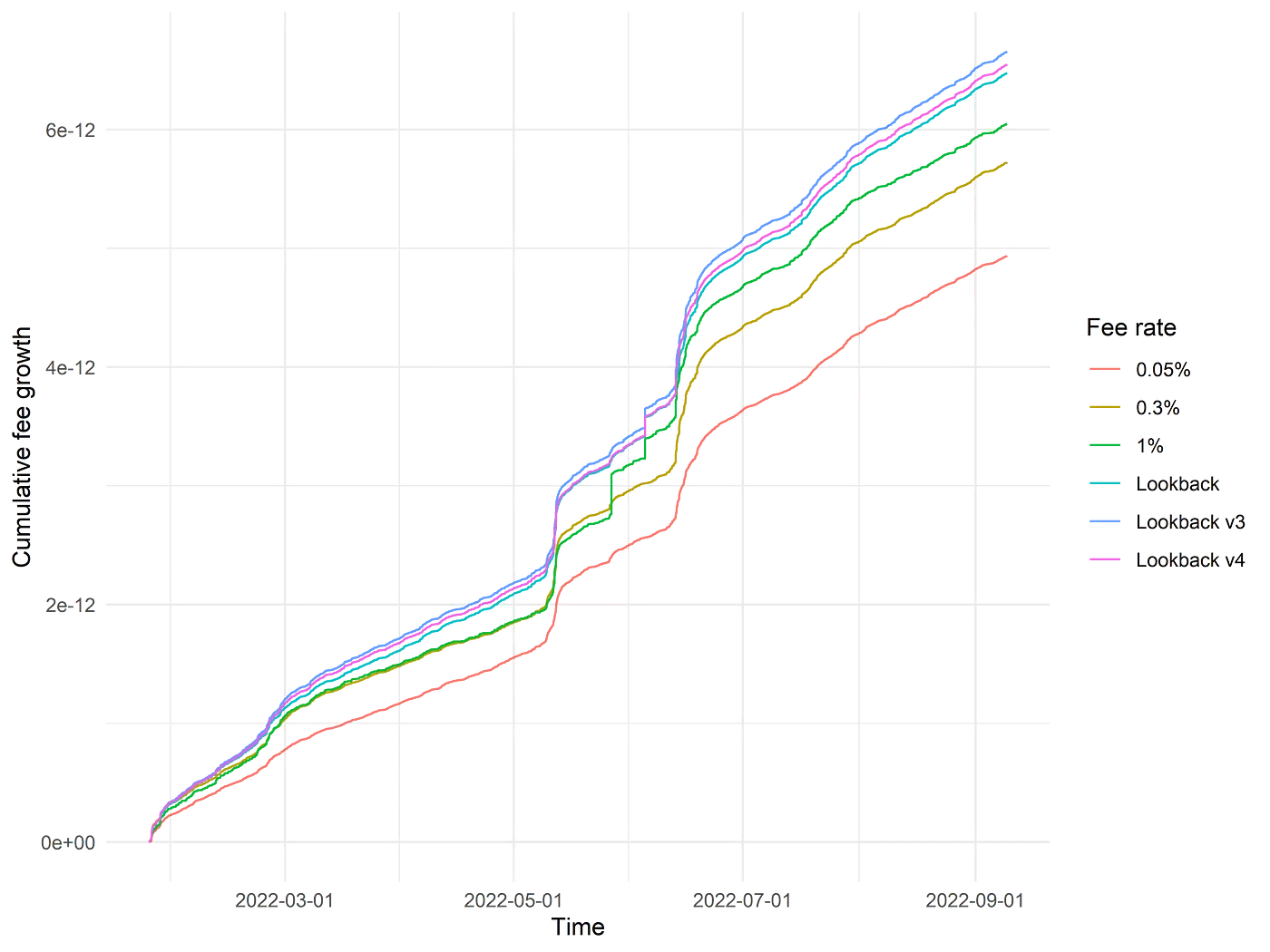
Plotting the backtesting results for the lookback v4 approximation via offsets, multivariate model and the normalized multivariate model yields the following results. The improvement from the normalization of the variables seems to be indistinguishable from the unnormalized model whereas the performance over the lookback/offsets is a modest improvement. 

All of the fee collection improvement is immaterial if the LPs are not compensated for the Impermanent loss/LVR that they bear for providing liquidity. The key question here is whether or not liquidity provision can be made into a consistently profitable endeavour net of impermanent losses (IL). Subtracting impermanent loss from fee accrual of the final linear model with daily retraining (not monthly) and calculating the cumulative portfolio growth in USD the team was able to generate promising results. 

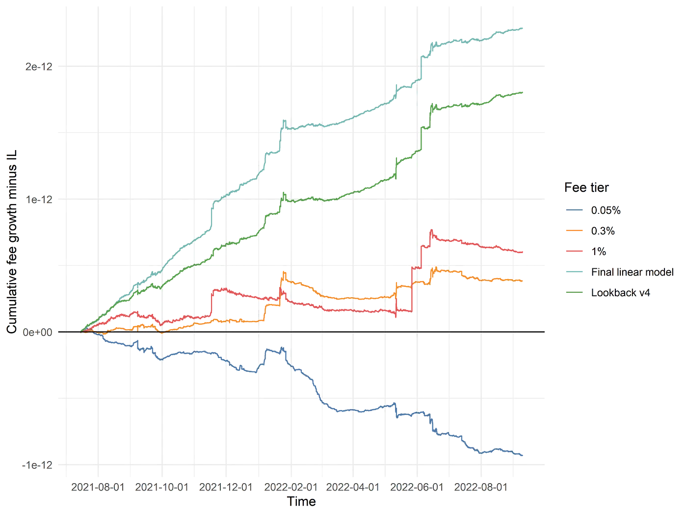
 On examining the plot, we find that all static fee portfolios throughout the entire dataset do not perform very well and have significant periods of underperformance. The performance enhancement of even the lookback model shows the benefits of switching to a dynamic fee setup. We can also see certain areas where the simpler lookback model failed to “react” appropriately to capture the temporarily elevated fee growth, but the multivariate linear model captured a great deal of the outperformance.

Volatility adjusted Fee AMM

Source: AMM 2.0 — Volatility Adjusted Fee

The basis for this design lies in the idea that a constant fee is inappropriate for different asset pools with different realized volatilities. Volatility-adjusted fees can potentially ensure that the Liquidity Providers (LPs) are fairly compensated for the risk they assume when providing liquidity across different market conditions and pools.

We now build a Volatility adjusted AMM step by step by trying to define various AMM parameters as functions of trading volume, TVL and variance of asset prices:

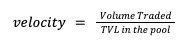
Step 1: Measure ‘AMM velocity’ as f(Trading volume, TVL)

AMM velocity is a measure that helps us understand the utility and efficiency of the assets being deposited in the liquidity pool. 

Step 2: LP wealth as f(Variance) in no fee environment

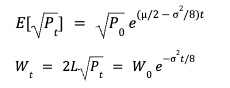
LP provides liquidity to a constant-product AMM pool in tokens X(e.g. ETH) and Y (e.g. USDC) and measures wealth in Y. Treating Y as numeraire, we have marginal price P_t = Yₜ/Xₜ and XₜYₜ= k = L² from the constant product invariant. Xₜ and Yₜ denote the LP token balances and L is a constant denoting liquidity supplied by the LP. In the absence of fees, LP wealth in the pool (Wₜ) is given by:

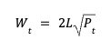
From the discussion about LVR in the previous post, we know that the square root of price follows a geometric Brownian motion. The drift = μ/2 - σ²/8 and volatility = σ/2. The expected value of the square root of the price at time t is given by:

By assuming the asset price drift 𝜇 = 0, we can see that LP wealth decays with ⅛ the variance of the asset price.

Step 3: AMM fee pricing as f(Variance, AMM velocity)

The fees on an AMM pool should be adjusted dynamically to compensate for the decay in LP wealth over time.

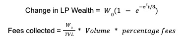
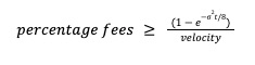
To attract LPs to provide liquidity for an extended period, Fees collected ≥ Change in LP wealth. By comparing the above equations we can determine

Further decisions that need to be made about this mechanism design include:

1. What is the right variance value to use in this model?

Due to the absence of a liquid options market for a majority of AMM pairs, we cannot use implied volatility from the options market. The Hydraswap team suggests using an exponentially weighted moving average (EWMA) variance. Using EWMA variance as a predictor makes use of a well-studied observation in finance called volatility clustering i.e. large variations in prices tend to be followed by large variations and small variations tend to be followed by small variations.

The fees need to be updated quickly enough to provide LPs with the opportunity to capture more fees in a volatile period or lower fees in periods of low volatility to remain competitive but it shouldn’t be recalibrated too frequently as it may increase the gas cost for swappers/liquidity providers. The team utilized hourly variance data for their backtests.    

We can also optimise the 𝜆 value (i.e. weight associated with past variance) for EWMA by calculating the point of least Mean squared error of EWMA and the actual variance noted in the period.

2. Estimating velocity for AMM major pools?

We can either calculate velocity on a per-pool basis or a global level across DeFi. For simplicity, global DEX data can help us decide on a fixed velocity parameter. Using historical trading data across major DEXs we can find the historical daily velocity i.e. average daily volume (ADV) to TVL in DeFi has averaged around 10%.

3. What are the fee ranges for liquidity pools?

An uncapped fee range can drop the fee down to 0% benefiting arbitragers and leading LPs with major impermanent loss or drive the fees to 100% leading to the swappers losing all their assets. Thus we need to define a minimum/maximum range of fees for each pool. Hydraswap team had opted to choose a range of 5bps to 200bps for their pools.

Backtest Results

Sharing the results of ETH/USD backtests done by the Hydraswap team - using 1-minute tick data from Binance to compare the performance of LPs. The constant fee is set to 0.3%, in line with major AMMs and all trades are considered to be informed trades (i.e. when profits from the trade exceed the fees paid). 

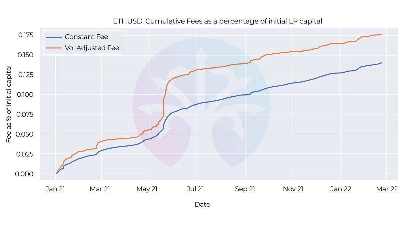
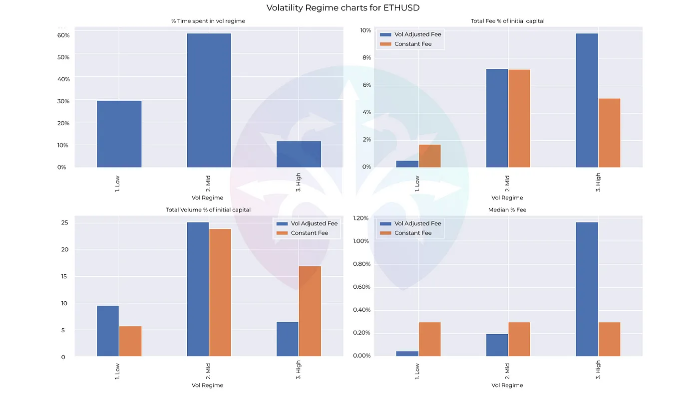
For ETHUSD the returns for LPs were 1.26x vs. constant fee strategy. The above charts show the behaviour of the two models in different volatility regimes {low (annualized vol<50%), mid (50%-150%) or high volatility (>150%)}.

Observations

1. Markets have low volatility for the majority of the time, with high volatility periods occurring only 10% of the time for ETHUSD during the backtest window.
2. The vol-adjusted fee pool traded lower volumes during high volatility periods but collected more total fees compared to the constant fee pool.
3. During low to mid-volatility periods, the vol-adjusted fee pool traded higher volumes than the constant fee pool and collected similar total fees.
4. The vol-adjusted fee model protects liquidity providers during volatile times by offering higher fees and encourages higher trading volumes by reducing fee rates during calmer market environments.
5. The median fee charged by the vol-adjusted fee model is significantly lower than the constant fee model, indicating its effectiveness in different market conditions.

Constant volatility AMM

This design stemmed from a couple of interesting observations made by @guil_lambert about the market pricing volatility similarly across fee tiers.

1. The 0.05% fee pool is perfectly suitable for ETH-stablecoin pairs, it seemed that the yields for the 0.01% pools were insultingly low with median LP fees in the 0.01% pool being about 0.005% of the deposited amount.
2. Even though the feeTier, the daily volume, and the amount of liquidity locked in a pool do vary quite a bit between pools, it appeared that the “market” has figured out a way to distribute that liquidity to maintain constant volatility between pools.

E.g. ETH-USDT pools all have similar implied volatility

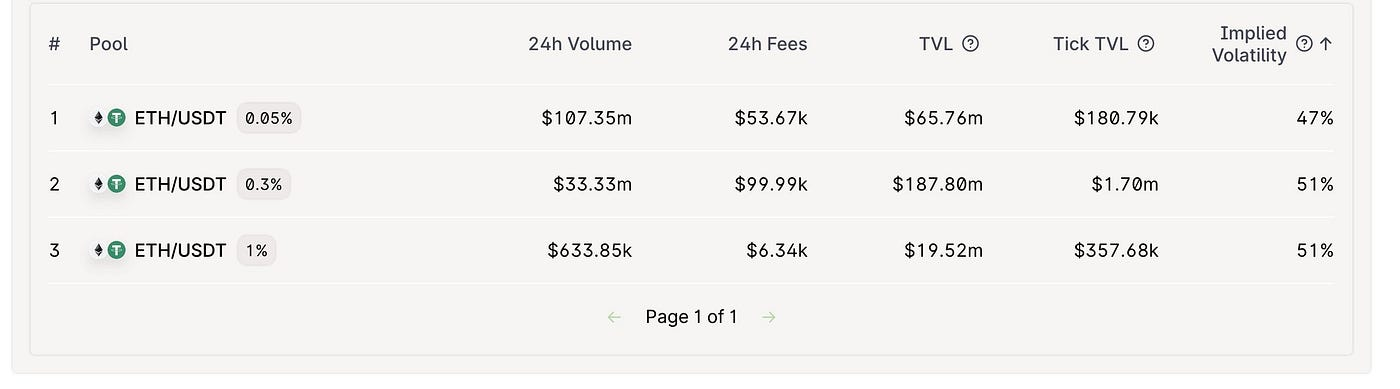
3. The yield should over time be the same across fee tiers because average returns are directly related to the volatility of an asset. This happens because rational market participants will recognize this will relocate liquidity from low volatility pools (ie. pools with low volume OR too much liquidity) to high volatility pools to maximize their yields.

The mechanism stems from building a responsive fee and constant Volatility AMM.

Step 1: Volatility as a function ~ f(fee tier, daily volume, TVL)

Assuming that the Efficient Market hypothesis holds for a majority of asset pools created on AMMs, most LPs would tend to lend their liquidity position instead of providing them to AMM pools if it is profitable to lend a Uni v3 LP position as an option instead of holding it. Thus the return from holding an LP position should be comparable to the premium collected by lending out/selling an option

To compare these 2 quantities we need to calculate them using common parameters.

1. Returns (Holding LP position): Guide for Choosing Optimal Uniswap V3 LP Positions
2. Returns (Lending option)/Premium approximation: Quant Finance Stack Exchange

Returns (Holding the LP position) = Returns(Lending the option)

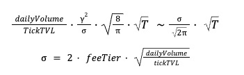
Where 𝛄 = fee Tier

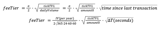
Step 2: feeTier as a function ~ f(TVL, daily volume, constant volatility)

By extending observation 2 about similar volatility for asset pools across fee tiers, we can make the argument that returns for LPs should be the same across all fee tiers as long as each pool follows the same asset. At the same time, we can postulate that we can achieve this in a variable fee environment by inverting the IV expression so that the feeTier depends on liquidity, and volume while keeping the expected volatility constant.

Basing the fee tier on the daily volume is perhaps a bit arbitrary. We can compute the feeTier on a per-trade basis too by setting the “time” variable to the time since the last transaction, and the trade size as amount0 (Trader wants to swap amount0 of token0 for amount1 for token1):

By fixing the volatility (e.g., IV = 100% annualized), we can arrive at the dynamic fee using the above expression. This calculation has interesting but non-intuitive consequences:

• More time between transactions: Leads to Higher fees
• Larger trade size: Leads to Lower fees
• Higher liquidity at the traded tick: Leads to Higher fees

Backtest Results

Working with a snapshot of the ETH-DAI-0.3% pool, the value locked at the spot price tick was 316 ETH and the implied volatility at that tick was 56%.

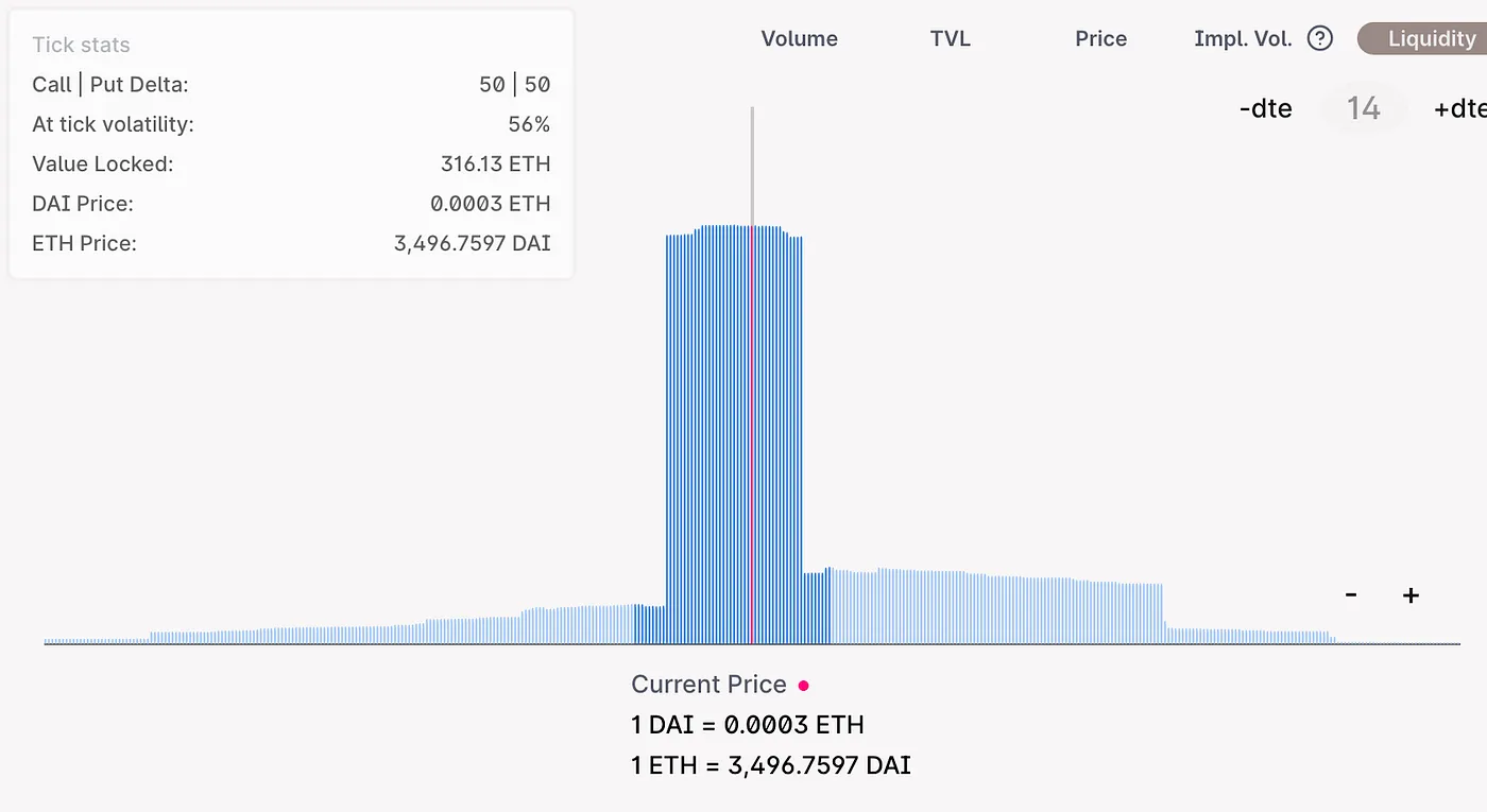
If one trade happens every block (blocktime=12s) and the pool targets an annualized volatility of 100%, then the purchase of 1 ETH would result in a fee equal to √12/11231 * √(316/1) = 0.58% i.e. About twice the normal fee.

Waiting for another block would increase this fee to 0.86%, with a general formula for the 1 ETH transaction being 0.58% * √(no of blocks since last transaction). However, if a whale instead sells 1000 ETH. Then the fee would be 0.02%, generating only 0.2ETH in trading fees for the liquidity providers. The slippage on that trade would also be 3 ticks for a ~0.9% slippage, so LPs would only collect 0.067ETH at each tick collectively.

Benefits and Tradeoffs of this Design

1. This design incentivizes more frequent and larger trades which in turn contributes to bringing the IV of these pools up and contributes to fee income.
2. For large trades, LPs collect lesser fees than fixed fee AMMs but at the same time, slippage can be arbitraged back to market prices cheaply on this AMM. So even though the effective fee was less than that of existing AMM fees, such a fee structure can create a ripple effect of arbitrage trades thus leading to more volume.
3. As higher liquidity at a particular price tick leads to higher fees such an AMM pool would not receive as much order flow from routing algorithms of DEX aggregators and routers which have support for the fixed fee pools with similar prices and liquidity distributions.
4. Fees in pools with long periods of inactivity (no trades) can become prohibitively expensive for swappers.

Flow-driven dynamic fees

Source: https://twitter.com/0x94305/status/1674857993740111872

This mechanism is built upon the simple observation that the fees of the AMM pool effectively define the bid-ask spread for that trading pair. Assuming that AMM price at a point in time is the same as the price on CEXes. Then, the AMM quotes a symmetric spread of 2*fees. The price of assets on the CEXs keeps changing. Suppose it goes up and jumps outside the AMM's bid-ask spread. Then usually, arbitrageurs will buy ETH from the AMM and sell it on CEXs such that ask prices on both the CEX and DEX match each other.  

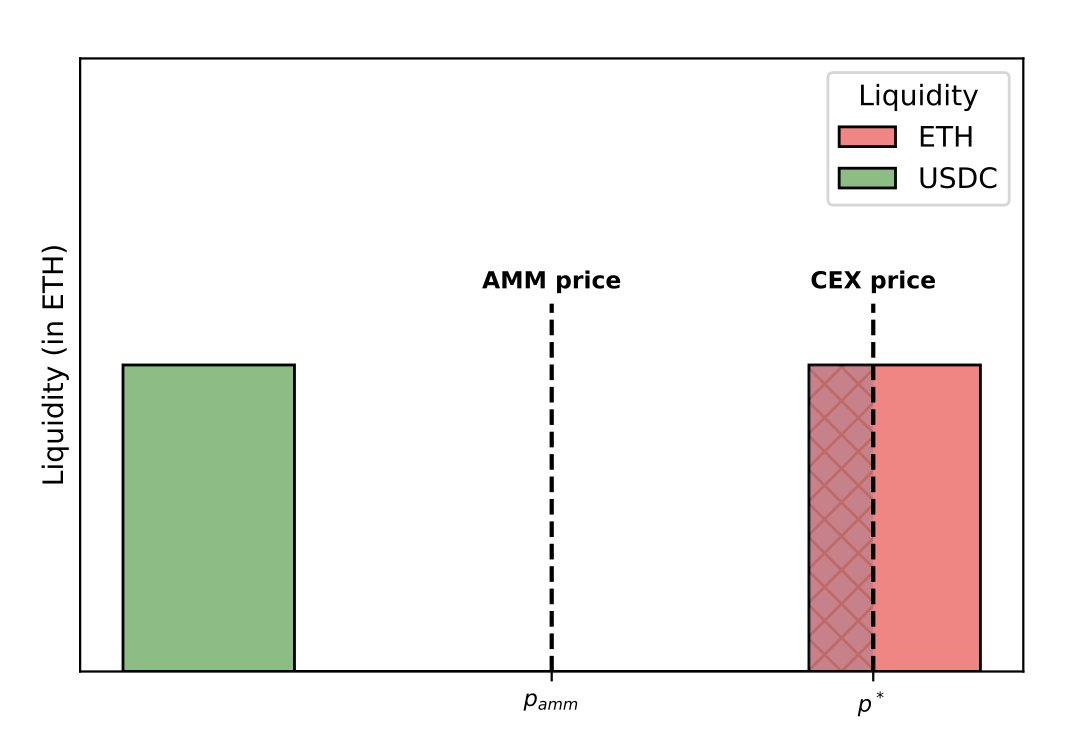
After the arbitrage trade, the AMM still quotes a spread of 2f. The best ask price on the AMM is now the CEX price, while the best bid is 2f away. The ask side of the book is more likely to get picked off again in case the price increases further on the CEX. The bid side is very far from the asset price (i.e. the quote on the CEX).

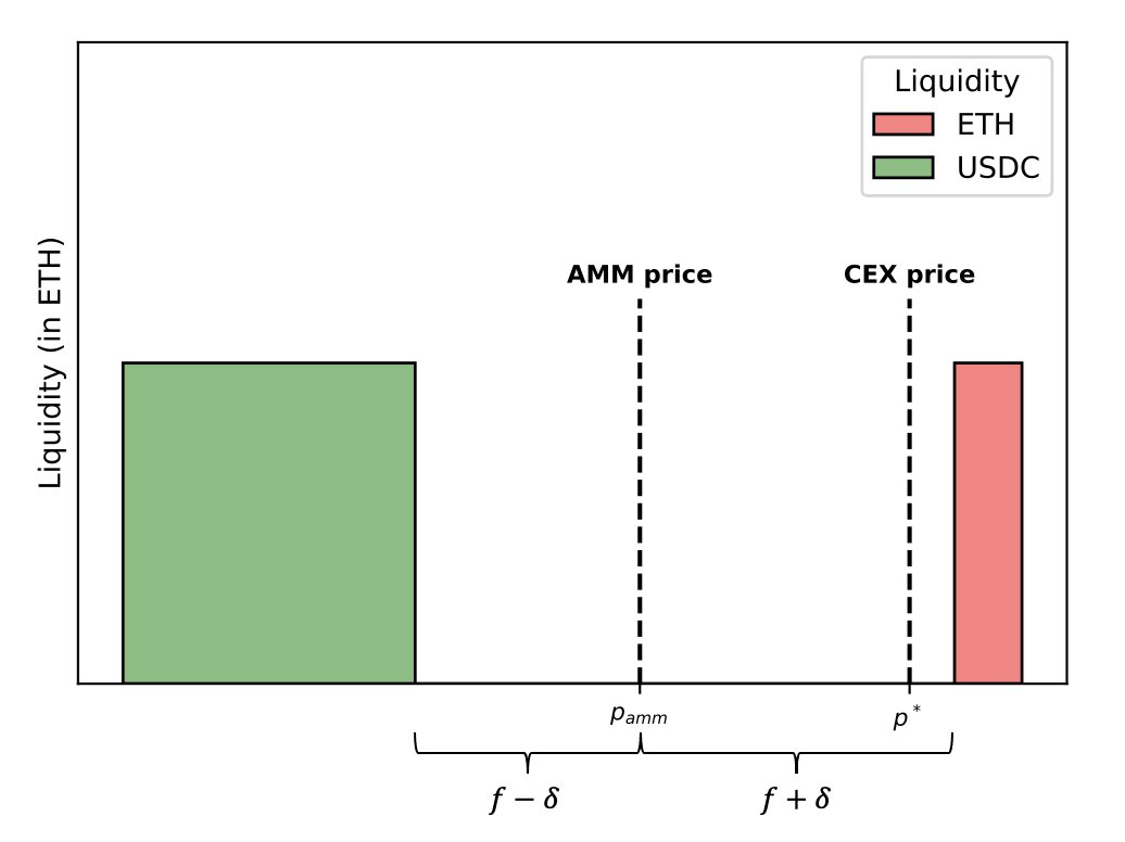
The suggested fix for this is to move both the bid and ask prices to the right - closer to the CEX price by a factor of 𝛿. 

1. Move the bid closer to the AMM price by 𝛿 - equivalent to reducing sell fees by 𝛿
2. Move the asking price further away from the AMM price by 𝛿 - equivalent to adding buy fees by 𝛿

As a consequence of this minor change in the AMM pricing function, we get:

1. The total spread quoted in the next block is still 2*fees
2. AMM can discriminate the arbitrage and uninformed flows as the direction of Arbitrage flow (unlike uninformed flow) is correlated and if the market price is pushing the ask it will more likely keep pushing the market price even further.
3. By moving the fee by 𝛿 the AMM can penalize transactions in the direction same as the previous transaction/block which is more likely to be Arbitrage traders (toxic flow) rather than uninformed traders. 

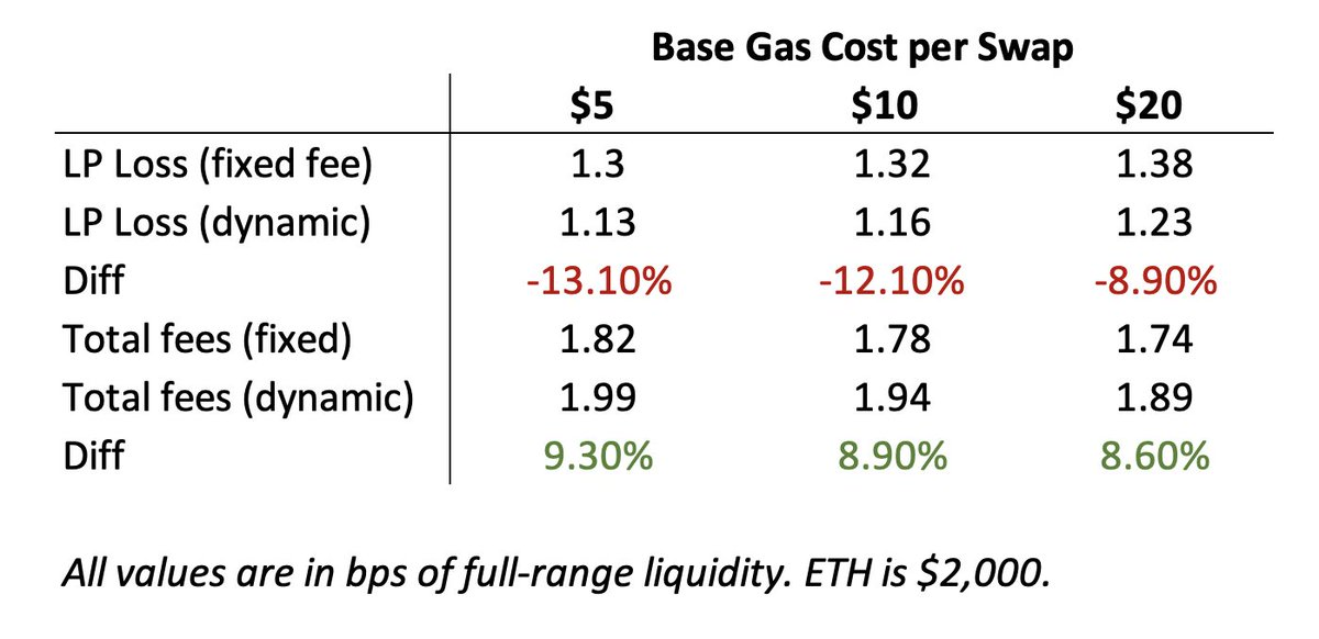
Backtest Results

Alex Nezlobin (@0x94305) shared a model of an ETH/USDC pool with $50,000 liquidity per basis point, 5 bps fee and 5% daily volatility. For each block, the fees are changed by 0.75 of the price impact of the previous block (𝛅 = 0.75 * price impact in previous block). The losses of LPs are about 10% lower with the dynamic fee than with a fixed one.

Curve V2 dynamic fees

Curve V2 was designed to provide deep liquidity for a wide range of assets with varying volatility. V2 requires the pool creator to provide values for a variety of tunable parameters that are used to optimize trading pools for different types of assets. An important feature of the V2 protocol design is dynamic fees for the dual purpose of - boosting LP fees and incentivizing the rebalancing of the pool to their internal price oracle. All Curve v2 pools consist of three core components: 

1. Bonding curve
2. Price scaling mechanism
3. Fee mechanism - parametrized by 3 parameters (fee Mid, fee Out, fee Gamma)  

Curve v2 pools charge a simple variant of dynamic fees depending on pool balance/imbalance. Fees are minimal when the pool is in a balanced state i.e. assets held are in their ideal proportion, and increase with increasing imbalance from this equilibrium.

Dynamic fees are defined using three parameters:

1. Fee Mid: The fee charged when the pool is completely balanced. This is also the minimum fee charged for any swap against the liquidity of the pool.
2. Fee Out: The fee charged when the pool is completely imbalanced. This is the maximum fee.
3. Fee Gamma: This parameter decides how quickly fees increase with greater imbalance. Lower values produce sharp fee increases with increased imbalance; higher values produce more gradual fee increases with increased imbalance.

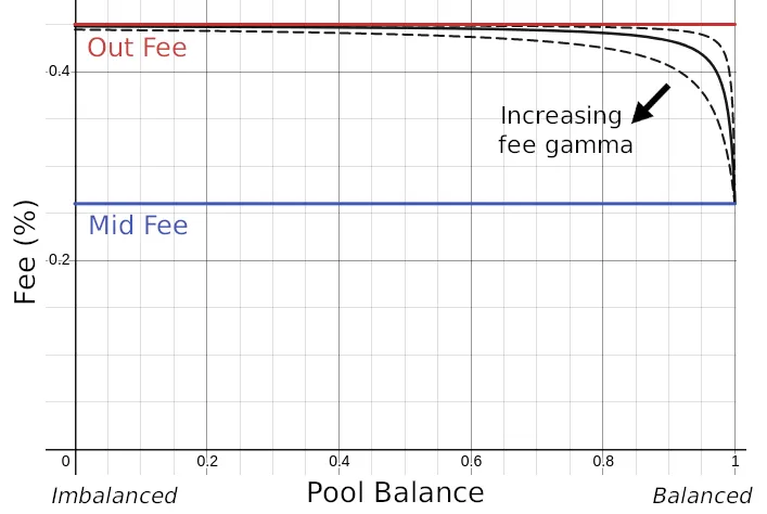
As the pool goes from fully balanced (x = 1) to fully imbalanced (x = 0), fees increase from mid-fee to out-fee. The rate of fee increase is controlled by the fee gamma parameter. 

As we can see this design leads to low fees in a balanced state attracting more traders to Curve pools and increasing fees to compensate LPs in cases of lopsided movement of assets from the pool (i.e. in an imbalanced state). These dynamic fees seem extremely basic compared to the other models we’ve looked at in this article but they also serve an integral purpose in the price scaling mechanism.

V2 pools dynamically shift liquidity to maximize depth and minimize slippage near current market prices. This is accomplished by taking a running EMA (exponential moving average) of the pool’s recent exchange rates (internal oracle) and re-centering/re-pegging liquidity at the EMA only when it is financially reasonable for LPs to do so (divergence loss which becomes permanent in this re-pegging doesn’t exceed half the profits made by LPs via fees).

Price where liquidity is currently maximally concentrated: Price Scale 

Current EMA price calculated from latest trades price data: price Oracle 

We can conversely think of this process as if the difference between the price oracle and price scale is larger than a minimum threshold then we check for profits generated by LPs. If these profits are greater than 2*realizable divergence loss then we re-peg the pool to oracle price.

In a situation wherein, profit < 2*realizable divergence loss:

Case1: Price differential continues to increase

The dynamic fees will gradually increase to accelerate the growth of the profit variable (i.e. fees) to the point where it becomes feasible to re-peg the pool

Case2: Price differential decreases

The oracle price will converge towards the price scale reducing the realizable divergence loss to the point of profit > 2*divergence loss or bringing the price differential below the threshold of rebalance.

Side Note: The Curve Finance team recently shared simulations on optimizing the dynamic fee and bonding curve parameters to increase the APY that LPs receive in the tricrypto pool. Results show maximum volume and minimal slippage occurs at out_fee=3% when mid_fee=0.03% with an APY of 44% (10x of current APY at the best conditions.)

We highly recommend reading through it as discussing the simulation would go beyond the scope of this article. 

Dynamic fees based on flow identification

As we already know LP losses occur due to toxic flow (arbitrage flow) that the LPs are exposed to in passive liquidity provision. If we can identify between uninformed and toxic flow and charge fees based on such an identification we can clawback a fraction of the LVR losses. 

The following are a couple of ideas that can be incorporated into AMM design 

1. Utilize an optional time delay acceptable to users to identify flow type. 

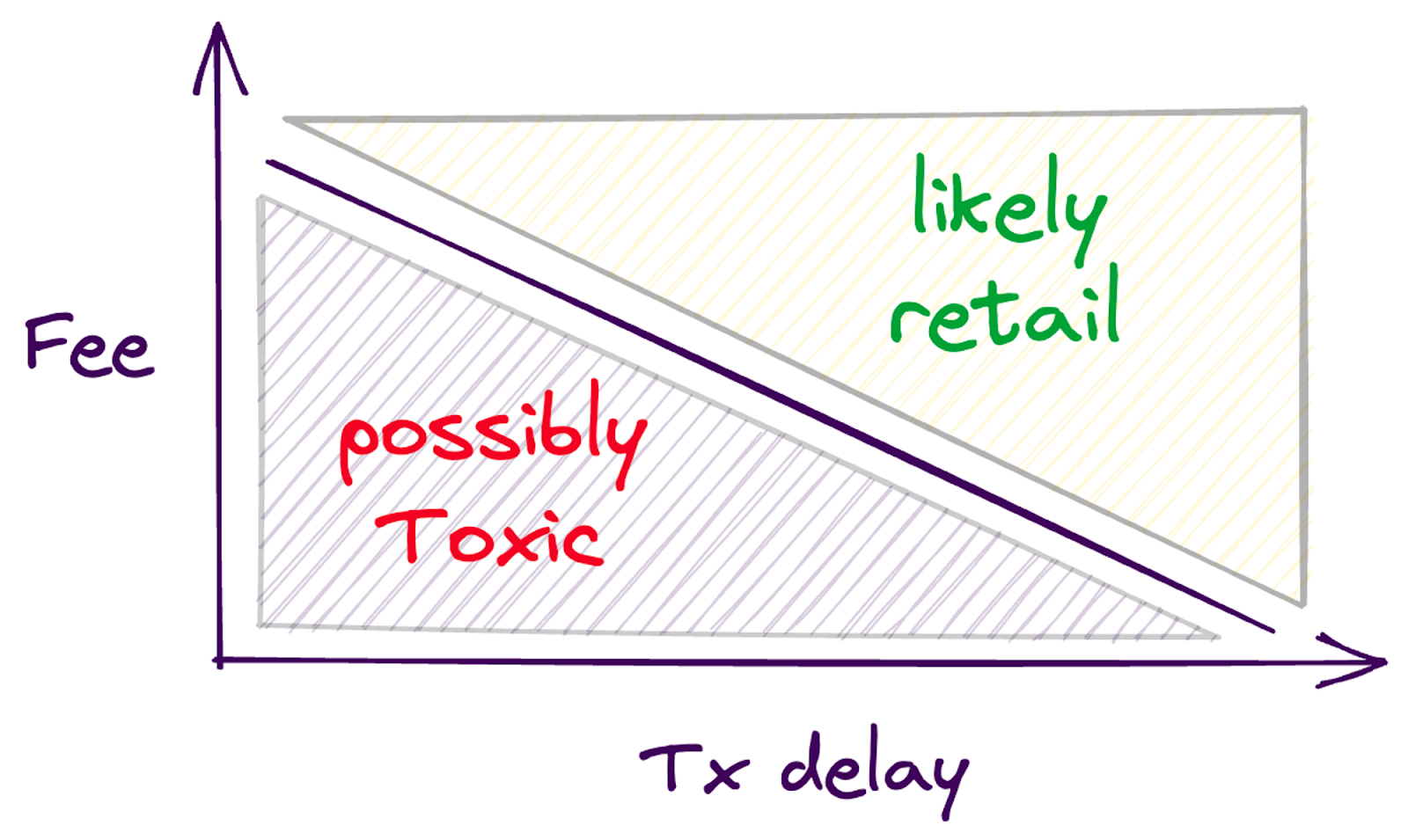
Trading signals and arbitrage opportunities decay rapidly, making it difficult for informed traders to catch the Automated Market Maker (AMM) off-guard with significant delays in order execution. Here's how such a mechanism could function:

1. Slow settlement is cost-effective: Users can opt for a low-cost swap (e.g., 0.1% fee) if they can wait for their trade to settle in 5 minutes. Uninformed traders find this option appealing, saving on fees while incurring minimal waiting time.
2. Fast settlement comes at a premium: Settling at the current Oracle price is expensive (e.g., 0.5%). A higher fee reduces the likelihood that an informed trader's signal advantage will be profitable for the AMM. This provides a quick settlement option for users willing to pay extra.

A delay enables the DEX to differentiate between toxic and non-toxic flows and adjust fees accordingly. To effectively block toxic order flow, fast settlement fees must consider the market volatility of the trading pairs. Another design example that utilizes a time delay for pricing adjustments to discourage arbitrage flow can be found in the design of Mooniswap by the 1inch team.

In a similar vein, Balancer governance vote reduced swap fees by 50-75% for all order flow originating from CowSwap. CowSwap employs batch auctions, which introduce a delay that deters toxic flow, allowing Balancer to lower its fees and increase profits for its Liquidity Providers (LPs).

2. Differentiate order flow on the basis of trade size

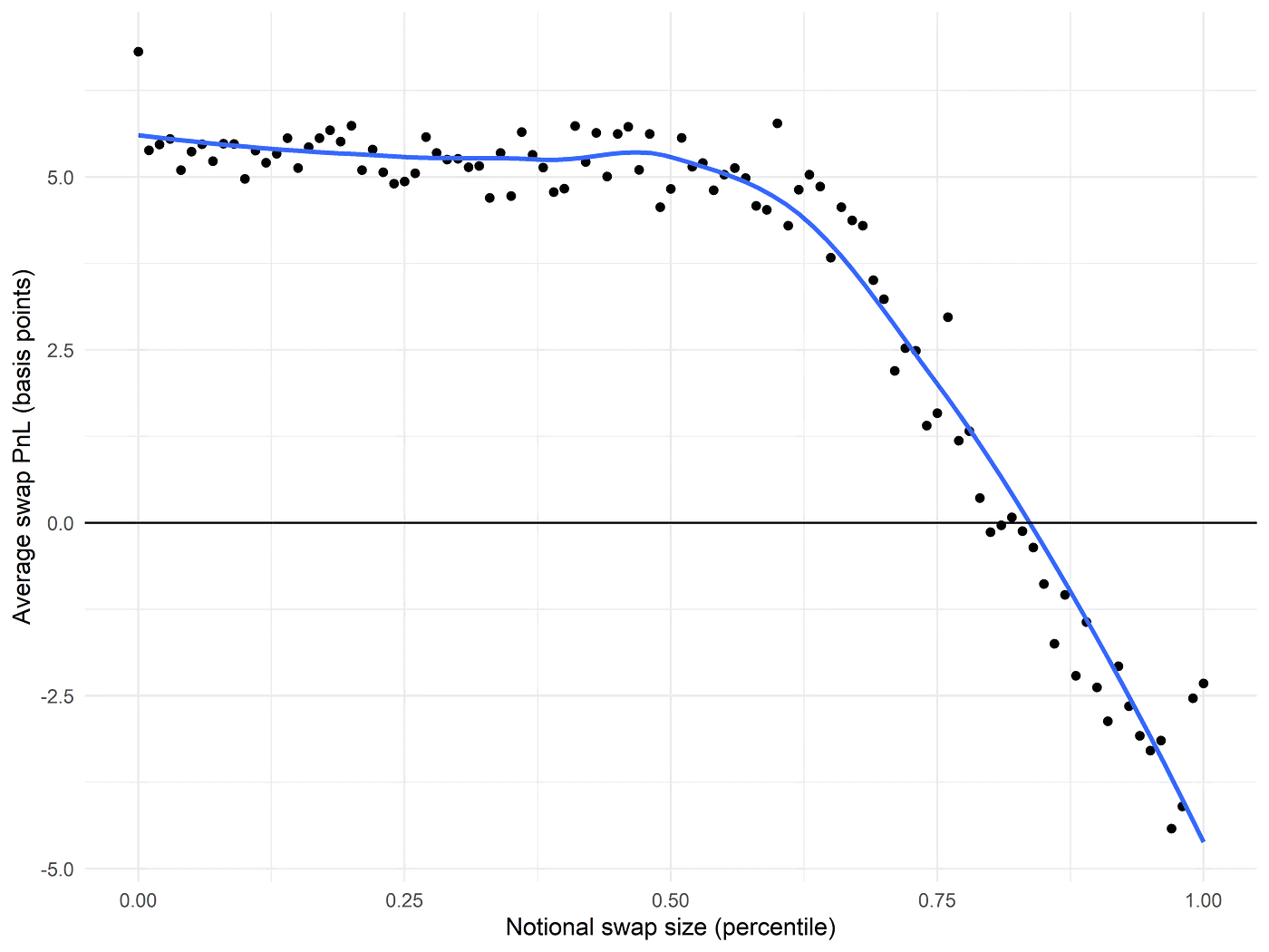
LP Profit drops off sharply as notional swap size in USD increases (using markouts to measure profitability). Interestingly, most of the pools’ losses come from swaps with a large notional size. Even though most swap sizes correspond to positive average returns (for the pool and its LPs) because the larger notional swap sizes correspond to negative average returns, liquidity providers’ end up with negative overall returns.

This observation motivates the idea of flow discrimination via swap size: 

What if the liquidity pool could preferentially charge higher swap fees to incoming swaps with a high notional size of each swap and increase the fee enough so that at the very least the expected PnL of the swap is zero for LPs.

However, an obvious problem with such a design would be that incoming swaps can be split up over multiple swaps or contract calls, so if it becomes known that the notional size of the swap is the determining criterion for the application of an additional swap fee, then swappers will be able to easily dodge this fee.

3. Differentiate orderflow based on the number of swaps originated from the wallet

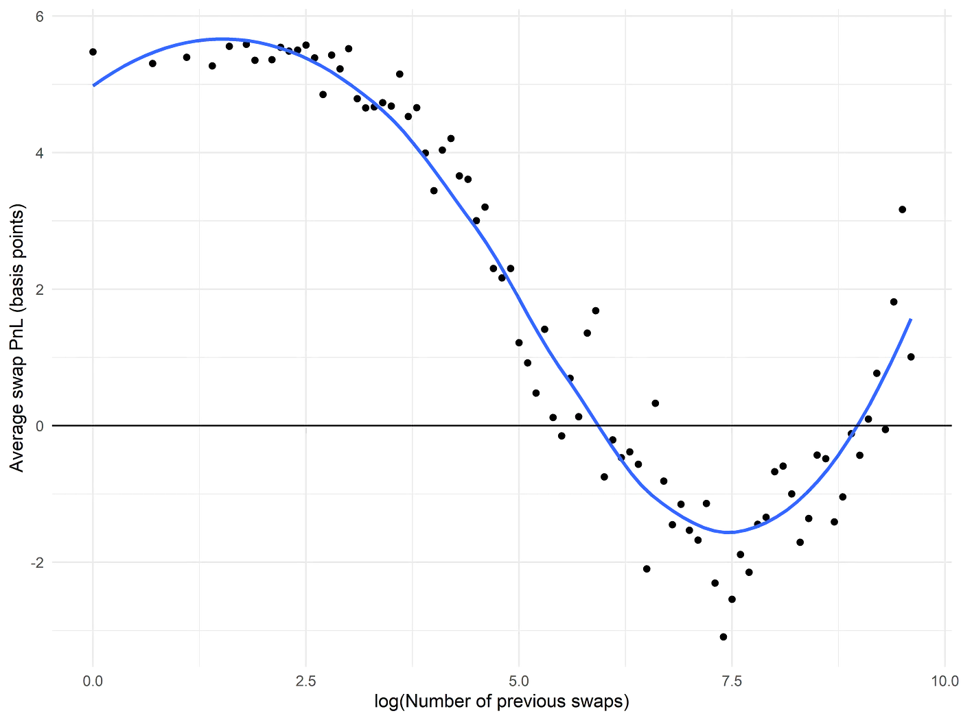
We see that wallets with relatively limited swap history are indeed likely to give rise to swaps that are profitable for the liquidity pool, i.e., their swaps are likely to constitute nontoxic flow. It is only when we see a swap history of ≥ 40 swaps that the average markout profit and loss begins to decline, reaching negative returns for swaps coming from wallets with ≥ 500 previous ETH/USDC swaps.

Curiously, we see that for wallets with quite extensive ETH/USDC swap histories, the expected PnL returns to positive levels. The Ambient finance team have discussed these 14 outlier addresses in detail in their blog post.

A simple strategy for determining fees would include providing lower fees for wallets that have not originated over 40-50 swaps over their lifetime and charge higher fees from wallets with 500+ swap transactions. The issues with such a mechanism is that it isn’t sybil resistant i.e. an arbitrageur could easily mask themselves by creating new addresses on a recurring basis. At the same time, it is valuable to note that:

• Moving assets between wallets will cost both time and money and incurs significant additional logistical complexity for arbitrageurs.
• Stricter criteria can be established for wallets to “qualify” as non-toxic flow. Example, a fee discount can be given to wallets that have swapped more than 10 times, but fewer than 1,000 times, in the ETH/USDC pool with average positive PnL for the liquidity pool. In other words, we can explore ways to make it prohibitively hard for toxic flow to “pretend” to be non-toxic flow with sophisticated checks.

Critique of dynamic fees

Originally discussed by Mallesh Pai, an SMG mechanism designer, most dynamic fee mechanisms are initially designed with current trade flows in mind. However, once the fee structure changes, predicting the resulting impact on trade flows becomes challenging. This raises the possibility of the new dynamic fee system altering the routing of informed and uninformed trade flows through these pools, a concept rooted in the economic principle known as the Lucas critique.

Given the ongoing structural changes in the DEX ecosystem, particularly Uniswap's introduction of interface fees, it's likely that more traders will shift towards DEX aggregators with lower or no platform fees. This prompts important questions: Can dynamic fee pools attract trade flow routing when their dynamic fees are higher than those in fixed fee pools? Will these pools primarily be utilized during periods of lower dynamic fees? Furthermore, does a market-leading DEX with substantial volume and liquidity need to transition from fixed to dynamic fees to accurately assess the impact on LP profitability?

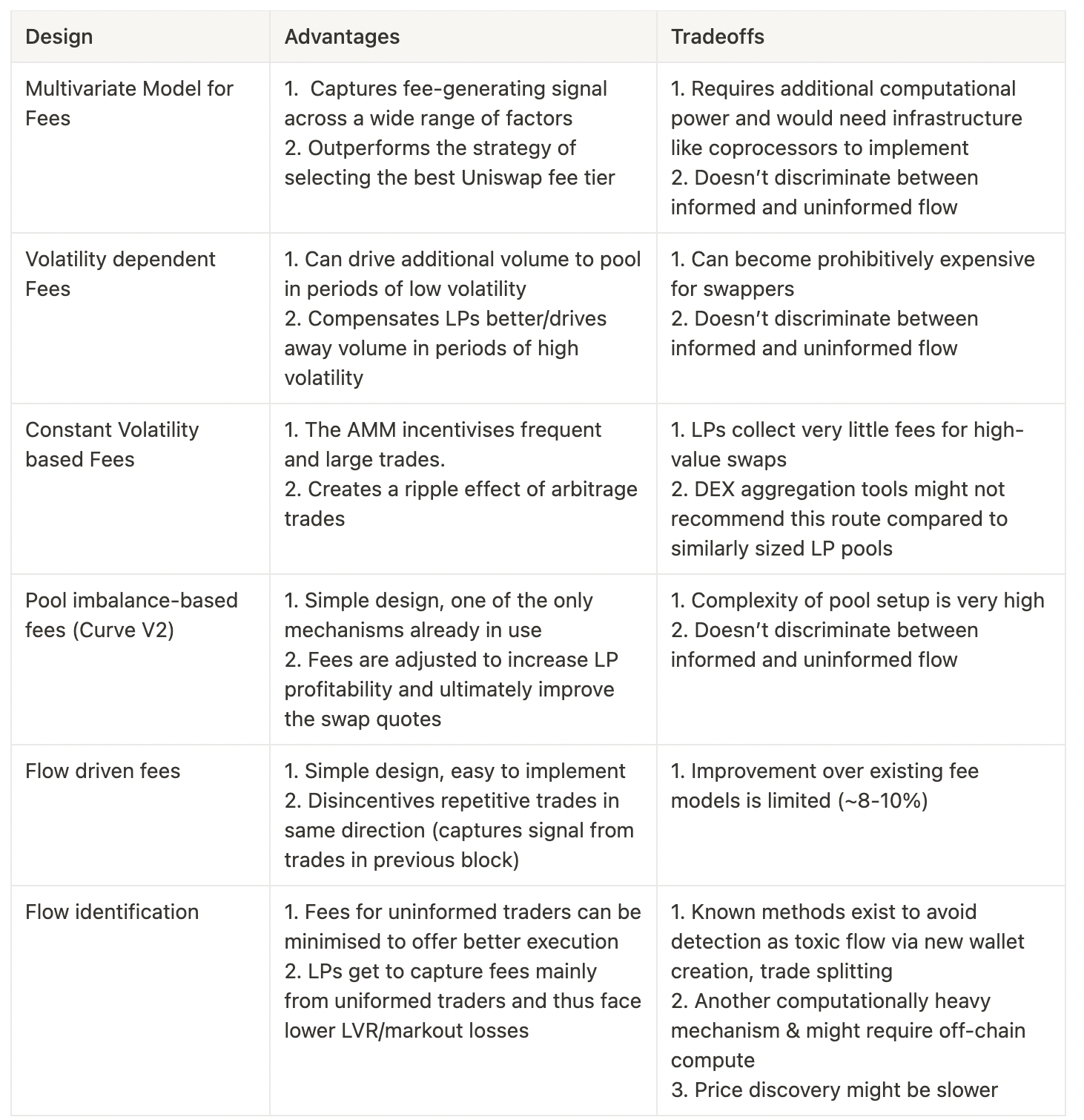
Conclusion

Summarising the various benefits and tradeoffs of the various mechanisms and AMM fee designs discussed in the article.

We believe that there are a lot of other potential dynamic fee implementations that we as an ecosystem can explore and experiment with to reduce the problems of LVR. Catalyst aims to leverage some of these leading dynamic fee mechanisms and is exploring additional mechanisms in order to preserve LP performance and profitability in its AMM implementation. 

We would be delighted to engage in a discussion with DeFi and AMM researchers interested in advancing the forefront of research on dynamic fees. In the upcoming articles of this ongoing series, we will be exploring other solutions for LP performance improvement such as hedging of LP positions, application-level improvements, protocol-level changes and the emergence of new infrastructure that will lead to the next iteration of profitable AMMs.

References

1. Constructing Multivariate Models to Improve a ETH/USDC Dynamic Fee Policy | by CrocSwap
2. A window into AMM 2.0 — Introducing Volatility Adjusted Fee | by Hydra
3. Designing a constant volatility AMM
4. Alex Nezlobin - flow driven dynamic fee system
5. Tricrypto dynamic fee parameters research and proposal
6. Deep Dive: Curve v2 Parameters - nagaking
7. The next steps in DEX design
8. Discrimination of Toxic Flow in Uniswap V3: Part 1 | by CrocSwap
9. Mallesh Pai - Lucas Critique for dynamic fees