Optimizing LP Performance Part 1: Metrics to measure performance

Cata Labs

Sep 18, 2023 • 17 min read

In DeFi, new innovations are forced to arise in order to operate within the constrained environment of on-chain block space. One of the most notable advancements has been the emergence and progress of Automated Market Makers (AMMs), which have transformed the way we trade and provide liquidity in DeFi. However, the evolution of AMMs is far from complete. As the multi-chain world continues to grow, we find that the existing AMM designs do not scale in order to meet the capital efficiency requirements and security standards for a thriving cross-chain economy.

Catalyst is not just another iteration of the existing designs; it is an AMM built from the ground up with efficient cross-chain swaps in mind. Existing AMMs have brought forth permissionless trading and liquidity provision, opening doors for easy swapping and pool creation within a single blockchain. Yet, Catalyst is being built for the next phase of this evolution, with the introduction of permissionless cross-chain and intra-chain swaps using the same liquidity.

While AMMs have reshaped how we interact with markets, the potential they hold is still bounded due to issues such as MEV leakage and degradation in LP performance (Liquidity Provider) it causes. We start this series of blog posts by building an understanding to solve these issues by delving deeper into the measurement of LP performance using a variety of metrics at our disposal - Impermanent Loss (IL), Loss versus Rebalancing (LVR), Fee Liquidity-Adjusted Instantaneous Returns (FLAIR) and Markout. By tapping into existing research on the performance of LPs both at the pool and individual LP level we aim to enhance and fine-tune the Catalyst AMM design.

This article marks the beginning of a series of articles that will delve into the intricacies of Catalyst's evolution, addressing the pressing challenges in AMM design right now, and looking to potential solutions that are pushing the boundaries of AMM capabilities.

In the upcoming instalments of this series, we aim to build an understanding of these solutions addressing critical issues at the protocol level and the application level.

Impermanent Loss

In constant function market makers, market-making incurs price change correlated market-making costs. This occurs as AMMs simulate a portfolio constraint. The composition of this externally modifiable portfolio is always composed such that it is worth the least compared to the market price. If the price of the past is different to now, the value of the current composition would be worth less than the value of past composition.

Very often this phenomenon is wrapped in a neat package called “Impermanent loss”. It can be viewed as an opportunity cost - if the price returned to the original price the cost would be 0 thus “impermanent”. In other words, Impermanent loss is the percentage loss an LP would experience for a given price movement from the prices where the LP provided liquidity. It is simply the difference between holding assets and depositing them in an automated market-maker-based pool for earning fees.

Constant product market makers (Uniswap V2 pools)

From the definition we provided earlier Impermanent loss can be calculated as

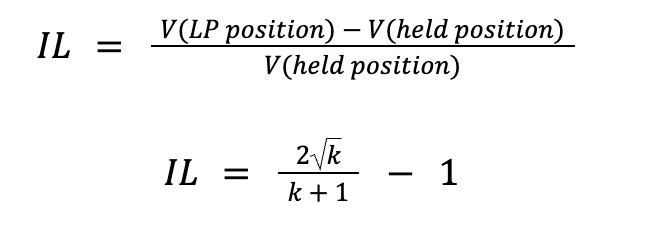
Where

IL: Impermanent loss

V(LP position) = Value of the Liquidity provider position

V(held position) = Value of assets deposited into the pool at current prices

k = constant defined as the ratio of new price/old price i.e. P’/P

The above formula doesn’t account for fees collected but we can adjust the formula for accounting the fees collected from the trading volume by adding the term fees(in USD)/V(held position). This formula has been derived many times in the context of AMM research and articles. For readers new to the concept of AMMs, the following article explains the derivation of the formula with examples.

Extending the above formula, Balancer’s multi-asset pools also follow a similar setup and a generalized formula for calculating the Impermanent loss for LPs in Balancer pools is as follows:

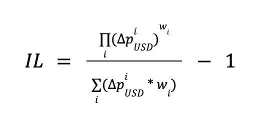
Where

Source: Balancer documentation

Concentrated liquidity market makers (Uniswap V3 pools)

Uniswap V3 liquidity providers provide liquidity in a fixed price range [a,b] via a feature called concentrated liquidity. With a concentrated position, reserves for both assets in the pool are consumed at a greater rate during trades leading them to be fully exhausted at either end of the range (a or b).

We can think about it as providing liquidity on leverage. If the price does not fall outside of the range, we can provide more effective liquidity. If the prices of assets in the pool exceed the range, the position is only left with 1 asset and not earning trading fees until the price reenters the range.

When trading on leverage, the gains and losses are amplified and the same is true for Uniswap V3. The trading fee share is higher for a concentrated position, however, the impermanent loss is higher too. We can come up with mathematical proof for how to calculate impermanent loss for these concentrated positions at price below, within and above the range of liquidity provision.

Where the range factor r = √(tickPrice_Higher/tickPrice_Lower) and 𝛼 is the current trading price of the pool. Interested readers can find the reasoning behind the respective formulas here.

Loss versus Rebalancing (LVR)

LVR is an alternative way to think about LP profit and loss, different from the Impermanent loss metric, but complementary to it.

The authors of the paper behind the metric start from the observation that impermanent loss (IL), i.e. trying to beat a strategy of holding assets, isn’t necessarily the best benchmark for LP profit and loss. In fact, IL mixes different two things:

Market risk: The position of the liquidity provider contains different proportions of the assets at all prices except the initial price of the position. Thus the pool position can overperform or underperform the holding portfolio due to the difference in exposure to market prices.
AMM-specific risk: This risk is a function of the trading function which in turn is related to the negative gamma of the position and the passive nature of the position.

The impermanent loss metric also discounts the path the price of the assets in the pool took to get from the initial to the final price. This becomes important as if the price oscillates sizeably then the opportunity to capture fees is also higher. The calculation of LVR stems from a basic equation to incorporate the fees collected and the path of price discovery:

LP Profit/loss = Rebalancing Profit/loss - LVR + Trading fee income

Simply explained, the metric is calculated from a benchmark portfolio that matches the LP’s asset composition but is being traded on a CEX. The idea is that whenever the price changes, the CEX portfolio sells one of the assets and buys the other in order to remain in sync with the composition of the LP assets and mirror the market risk. Intuitively, the rebalancing strategy buys exactly the same quantity of the risky asset as the CFMM does, but does so at the external market price, rather than the CFMM price.

This portfolio is also exposed to negative gamma (just like the original LP position) and is expected to lose compared with a non-rebalancing HODL portfolio. Loss-versus-rebalancing (LVR) is defined to be the difference in value between the rebalancing portfolio (Rt)and the CFMM pool (Vt), i.e.

$ LVR_t = R_t - V_t$

LVR is a form of “adverse selection”: it is an information cost paid by the LPs to agents with superior information (arbitrageurs with knowledge of external market prices).

LVR formulation

The authors introduce the concept of instantaneous LVR in order to measure the LVR for an asset pool over arbitrary time periods. This is understood as the LVR per infinitesimal unit of time. It’s directly proportional to

Price volatility squared (σ²)
The gamma of the LP’s position depending on the AMM’s trading function

An intuitive proof

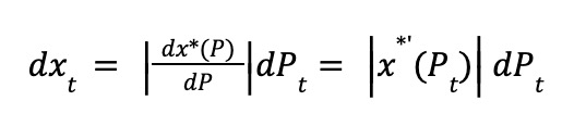
Suppose the market price changes from Pt to Pt+dPt. Arbitrageurs thus trade with the CFMM, moving from point A to point B on the CFMM invariant curve. Let dxt denote the amount of the risky asset sold, indicated by the green horizontal line. When the price moves from Pt to Pt + dPt, the rebalancing strategy sells exactly the same amount, dxt, of the risky asset as the CFMM does.

However, the rebalancing strategy trades at the CEX price, Pt + dPt. It trades along the brown line of slope Pt + dPt passing through A, and reaching point B*, which is higher than point B. Thus, after prices move, the LP position and the rebalancing strategy hold the same amount of the risky asset, but the rebalancing strategy holds more cash. The gap is equal to the height of the line connecting B and B* and is also the instantaneous LVR for the strategy.

To calculate the height of the B−B* line

Rebalancing strategy trades at the slope of the brown line, which is Pt + dPt
The CFMM trades at the slope of the purple line — that is the secant line connecting points A and B with a slope Pt + dPt/2

Thus, the B − B* line has a height equal to the difference in the slope multiplied by the risky asset traded

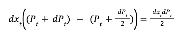
Now, we can write the amount traded $dx_t$ as a function of $dPt$

Thus, the instantaneous LVR

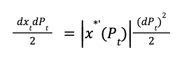
Using the assumption that price changes can be approximated as a geometric Brownian motion, in a small amount of time $d_t$, the quadratic variation $ dP_t^2 $ is equal to $σ_t^2 P_t^2)$, i.e. instantaneous variance $ σ_t^2 $ multiplied by the square of the price

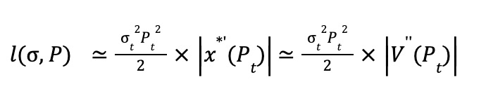
Integrating this instantaneous LVR over time [0,t] helps us calculate the LVR for liquidity providers of an AMM pool over a time period.

Further reading for interested readers: LVR with Fees

Example of LVR calculation

LVR can be defined on a trade-by-trade basis and thus we can look at a single trade. Consider a Constant Product Market Maker (Uniswap V2 style pool) with 1 ETH and 1000 USDC.

The market price of ETH jumps suddenly from $1000 to $4000.

AMM trading pool: A profit-maximizing arbitrageur will buy 0.5 ETH from the CPMM at an effective per-ETH price of 2000 USDC, thereby keeping the invariant (x*y) constant while moving the spot price to 2000/0.5=4000 USDC/ETH.

Rebalancing Portfolio: It will copy the CPMM’s trade (meaning sell 0.5 ETH) but execute it at the current market price of $4000 (on a CEX). This alternative strategy results in a portfolio worth $1000 more than that of the CPMM ($5000 vs. $4000), we can say that the LVR of this trade is $1000.

The price of ETH suddenly jumps back down to $1000

AMM trading pool: The CPMM will return (post-arbitrage) right back to its original state of 1 ETH and 1000 USDC, in effect buying back the same 0.5 ETH for the same per-ETH price of 2000 USDC.

Rebalancing Portfolio: Copies the trade (buying 0.5 ETH) but executes it at the market price ($1000). The market value of the rebalancing strategy’s portfolio is now $1500 more than that of the CPMM ($3500 vs. $2000), with the second trade contributing an additional $500 to the cumulative LVR.

Unlike impermanent loss, LVR depends on the price trajectory (LVR is 0 if the price stays constant but not if it jumps up and then back down) and accumulates on a trade-by-trade basis (as every trade might be on the wrong side, leading to additional adverse selection costs).

Fee Liquidity-Adjusted Instantaneous Returns (FLAIR)

LVR does not factor in a critical component of AMMs: the intra-pool competitiveness over other LPs that are in the same pool. LVR is not, in general, able to distinguish between high fee-return-on-capital and low fee-return-on-capital pools. FLAIR is a metric for LP competitiveness that supplements LVR, aiming to capture the dynamic behaviour of LPs within a pool.

FLAIR shows economically rational LPs will consider the cost and benefit of being an LP. This metric is measured in ex-post fashion – i.e. assessing the realized past performance (quantified through trading fees) within some time frame. In addition to general market risk, LPs must also consider how sophisticated their counterparty is. If a trader has better market information than an LP, the LP risks being on the wrong side of the trade and losing money.

FLAIR reflects reasonable economic intuition that LPs increase competition within pools by allocating capital to pools with higher fee returns, rebalancing in-range liquidity, and timing liquidity deployment to high fee periods. In short, LPs that frequently rebalance will earn more fees on average — a factor that is measured with FLAIR.

FLAIR will also be helpful for new LPs considering their participation in a pool and wants to assess the potential fee return on the capital they would have, had they followed the best strategy they could have out of the ones they have available (i.e., backtesting liquidity provisioning strategies).

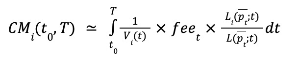
If the market value of the portfolio holdings of LP position 𝑖 at time instant 𝑡 is denoted by 𝑉𝑖(𝑡), and the pool’s spot price by $p_t$. Then the FLAIR for this position will be defined as

To generalize the calculation of the metric across Uni V3 type pools, we define arbitrary (discrete, potentially infinitely many, and arbitrarily fine) price intervals of the form [𝑝𝑘, 𝑝𝑘+1] for indices 𝑘 ∈ Integers.

In particular, we say that there exists a piecewise-constant liquidity distribution 𝐿(𝑝) that has the property that 𝐿(𝑝) = 𝐿𝑘 for all 𝑝 ∈ (𝑝𝑘, 𝑝𝑘+1) such that whenever the spot pool price 𝑝 ∈ (𝑝𝑘, 𝑝𝑘+1), the valid reserves (𝑥, 𝑦) contained in the pool satisfy the relationships 𝑥 = 𝑥*(𝑝, 𝐿(𝑝)) and 𝑦 = 𝑦*(𝑝, 𝐿(𝑝))

Calculation of FLAIR

Let’s assume that there exist positions in a pool such that the 𝑖-th LP has supplied at the time instant 𝑡, when the implied pool price is 𝑝˜𝑡, a liquidity distribution 𝐿𝑖(𝑝;𝑡) in the pool. A liquidity distribution is an entire function of price because the deployed liquidity varies with price. In total, the aggregate liquidity distribution in the pool is

𝐿(𝑝;𝑡) = Σ𝐿𝑖(𝑝;𝑡)

Denote by fee𝑡 the instantaneous fee rate earned by the entire pool due to all trades (i.e., both noise and arbitrage trades) at time instant 𝑡; in other words, ∫︀fee𝑡 𝑑𝑡 are the total fees earned by the entire AMM pool until time 𝑇. Finally, we note that, when the external market price of the risky asset is 𝑝𝑡, and the implied pool price is 𝑝˜𝑡 (where 𝑝˜𝑡 = 𝑝𝑡 if the

arbitrageurs are assumed to always trade until the external market price, irrespective of the trading fee, otherwise differing according to some bounded mispricing process), then the market value of the portfolio holdings of position 𝑖 at time instant 𝑡 will be

𝑉𝑖(𝑡) ≜ 𝑝𝑡 · 𝑥*(𝑝˜𝑡, 𝐿𝑖(𝑝;𝑡)) + 𝑦*(𝑝˜𝑡, 𝐿𝑖(𝑝;𝑡))

Following the aforementioned notation, we measure FLAIR for the existing LP position 𝑖 as

To calculate the aggregate pool competitiveness between different pools of assets (e.g. ETH/USDC 5bps pool vs ETH/USDC 30 bps pool vs AAVE/ETH 30bps pool), we can proceed with a modification i.e. 𝐿𝑖(𝑝;𝑡) = 𝐿(𝑝;𝑡) and thus calculate FLAIR across the pool

Example - Uni V2 style pools

To simplify calculations for the example case we make the following adjustments:

Consider that there are only 2 positions (LPs) in the pool, one is our “test” position (on which we are going to evaluate the metric) and the other one which will represent the aggregate of all other positions in the pool
There is a constant fee rate fee𝑡 = 𝑓 = 1 (Could be any other constant too)
For the realised price trajectory, we examine two cases:
Price remains constant throughout the examined time period
Price increases linearly increasing from 𝑡0 to 𝑇, such that

𝑝𝑡 = 𝑝˜𝑡 = 𝑝_min + (𝑝_max − 𝑝_min) · [(𝑡−𝑡0)/(𝑇 −𝑡0)] ∀𝑡 ∈ [𝑡0, 𝑇]

In the case of V2 styled pools, the entire curve does not exhibit concentrated liquidity, all LP positions have to be full-range, providing liquidity over the range (0, ∞). This restricts the set of possible LPing strategies to one. Two fully competitive LPs will place their liquidity into the pool at time 𝑡0 and make no adjustments, because adjusting cannot increase their competitiveness in the pool.

Case 1: Spot price of the pool remains constant

Suppose the test LP has contributed 10% of the total liquidity in the pool, then at any given point Vi(t) = 10% of V(t) and his/her liquidity distribution will account for 10% of the pool i.e Li(p;t) = 10% of L(p;t). As the price within the pool remains constant we can also consider $ V(t) = V(t) = c $ for some constant c.

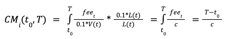
For the other LP position in the pool (Aggregate for all other LPs)

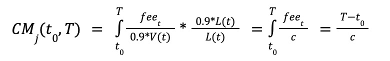
The result is very simple via modifications to V(t) extendable to case 2 (the price of the asset increases linearly). This confirms the obvious observation that in simple CFMMs with no active LPing, the instantaneous competitiveness of all positions remains the same through time. In other words, the competitiveness of LPs has no effect in this case, which is the expected behaviour. Even the variability arising from how much capital is deployed by a particular LP is, in aggregate, being abstracted away due to the normalization of return on capital.

FLAIR as a metric can be used by LPs to evaluate the best pools to deploy capital into by comparing the metric on an aggregate pool-to-pool basis. Thus the metric can help both active and passive liquidity providers to determine the best return on their capital across the large number of liquidity pools that are deployed on most CFMMs.

Figure: The top right batch of pools has low flow toxicity and low competitiveness of LPs. The bottom left corner has pools with high flow toxicity and high competitiveness of LPs (very dynamic strategies, active LPing, JIT liquidity).

Markout Analysis

Markout is a common metric used in high-frequency trading to analyze a strategy’s profitability. Imagining the Uniswap liquidity pool as implementing a trading strategy that takes the other side of every valid trade submitted to the pool we can calculate Markout for LP positions.

This Markout analysis was done initially by twitter user @thiccythot_ in his dune query analysing the UniV3 WETH/USDC pools. This sparked a debate between 0xShitTrader and members of the Uniswap team over the accuracy of the dune query.

Order flow toxicity via Markout is calculated by comparing the execution price to a future price or ‘mark’. Toxic flow is when the price marked to the future is worse than the execution price after accounting for fees and price impact.

$ m = d*v*(f-p) $

Where m = markout, d = buy (1) or sell(-1), v = volume and f=future price at time t, p=execution price

Some issues around the usage of Markout for measuring AMM LP profitability have been extensively discussed by traders and researchers. The team at Ambient finance have helped narrow down the major points of discussion for the Markout metric:

Swap fees should be incorporated into effective swap price

The swap price is computed from the number of tokens transferred to and from the swapper, as reported in the Uniswap event logs. These logs thus already incorporate the fees as Value[tokenout] = (1-fee)*Value[tokenin]
We calculate the effective execution price using the token in/out values, a higher LP fee will make it appear as though the swapper received a worse-than-market price, and conversely, that the LP filled the order at a better-than-market price.

The markout price should be the pool price

The original dune query is written using the logic that - For any given swap, we take the last swap performed in the next 5 minutes, including that swap itself if no other swaps occur.
However, this is potentially quite different from the price of the pool after the last swap was made. Eg. a pool with an ETH price of 1000 USDC/ETH will make sell ETH reserves leading to a new price of 1100 USDC/ETH. Thus an average execution price would be closer to 1049 (~√1000*1100) and the final pool price is 1100 a difference of US$50 for a 1 ETH swap.
We can thus see that the decision of using swap price or pool price for markout calculation can make a significant difference.

There should be no exit slippage

Although markout as a metric looks at the profitability of individual trades, it is almost always applied in the context of a continuous trading strategy.
Any trading strategy (including providing passive liquidity in an AMM) involves buying and selling inventory over a long trading period followed by an exit from the strategy. Calculating markout assuming exit fees on every single trade will be underestimating the strategy profitability.

Downward Bias of the Metric

If a given swap goes in the same direction as the last swap in its markout period (including itself), this means that the LP fee is exactly cancelled. e.g. a single swap in the period would display a markout = 0 but the LPs have collected swap fees which get cancelled out in this form of a calculation.
The directionality of swaps is typically correlated, and many likely intervals in which the markout period contains no additional swaps. As such, it can be suspected that this leads to a systematic underestimation of markout PnL.

We wish to measure optimal markout such that it captures as many microstructural properties as possible but as little asset price drift as possible. And to do so, the Ambient Finance team has made a few recommendations.

Recommendations from Ambient Finance to measure Markout

Calculating markout prices differently, first by using the price of the liquidity pool itself and, afterwards, by using Binance ETH/BUSD 1-minute candle opening prices.

A major problem with using Uniswap pool prices as markout prices is that only takers can change prices on Uniswap i.e. pool price on Uniswap tends to “lag” the fair price of the asset. There’s a cost associated with being a taker on a Uniswap pool (swap fee + gas cost), and arbitrage only happens if the arbitrage profits are greater than the cost of the trade.
This effect leads to an overestimation of LP profits when markout periods as low as 5 minutes are used.

Normalizing PnL of each swap by the number of liquidity units active at that time.

Moreover, the fraction of that liquidity which is active also varies dramatically e.g. 0.3% ETH/USDC Uniswap V3 pool, the proportion of liquidity units active in the pool ranges between 20% and 95%.
Impact of active liquidity fluctuations should not be understated. For example, imagine that a liquidity pool has net profits of -100 and +1 at periods 1 and 2, but that there are respectively 100 and 1 units of active liquidity at each time point.
Normalizing for active liquidity helps potential LPs analyze the performance of the strategy for each dollar of liquidity provided and the potential upside from actively managing liquidity.

The results of markout analysis using the 1. original method, 2. updating markout prices to final pool prices and 3. Using spot price data from Binance for the ETH/USDC Uniswap V3 pools aggregated across fee tiers are

Conclusion

As seen in the diagrams for metrics like Impermanent Loss and Markout analysis, the existing liquidity providers are suffering heavily from the problem of adverse selection. As discussed earlier, comparing the performance of LP positions to a buy-and-hold portfolio may not be an accurate way to assess the performance of these strategies. This is why we’re observing that metrics like LVR and FLAIR are finding increased adoption to gauge liquidity provider performance for both - asset pools and individual positions in these pools.

Significant product development and research have been conducted to mitigate and minimize the LVR for AMM liquidity providers. In the upcoming articles of this series, we will cover solutions for these issues at the protocol level and application levels. These include dynamic fee systems, consensus changes, methods to generate additional revenue for LPs, novel auction mechanisms and identifying and isolating toxic order flow.